Advanced recipes

This vignette gives some examples of more advanced/involved uses of STbayes.

library(STbayes)

Multi-network models

To create a multi-network model, you can just add more columns to the networks data-frame. Below is a toy data-set of two trials each with 3 individuals, and we define a kin and inverse distance network.

event_data <- data.frame(
    trial = rep(1:2, each = 3),
    id = LETTERS[1:6],
    time = c(2, 1, 3, 4, 2, 1),
    t_end = c(3, 3, 3, 4, 4, 4)
)
networks <- data.frame(
    trial = rep(1:2, each = 3),
    from = c("A", "A", "B", "D", "D", "E"),
    to = c("B", "C", "C", "E", "F", "F"),
    kin = c(1, 0, 1, 0, 1, 1), # first network
    inverse_distance = c(0, 1, .5, .25, .1, 0) #second network
)
data_list <- import_user_STb(
   event_data = event_data,
   networks = networks)

Individual-level variables (ILVs)

Individual-level variables can be either constant (e.g. age, sex) or time-varying (e.g. body condition). Below I define constant ILVs age, sex and weight to add to our toy dataset above.

ILV_c <- data.frame(
    id = LETTERS[1:6],
    age = c(-1, -2, 0, 1, 2, 3), # continuous variables should be normalized
    sex = c(0, 1, 1, 0, 1, 0), # Factor ILVs must be input as numeric
    weight = c(0.5, .25, .3, 0, -.2, -.4)
)

The data-frame ILV_c holds the values for each individual. The formatting of id should match the event_data and networks data-frames. At the moment, ILVs can be continuous or binary. You should normalize continuous variables, and binary variables should be coded as 0, 1. I plan to expand this to multi-category factors, but for the moment you must directly edit the Stan code to use these.

We need to explicitly tell STbayes which variables are additive (acting independently on intrinsic or social rates) and multiplicative (same effect estimated for intrinsic and social rates). Below, I have specified age as acting independently on the intrinsic and social rate, sex as acting only on the social rate, and weight as a multiplicative effect. Two betas will be estimated for age, and a single beta will be estimated for sex and weight.

data_list <- import_user_STb(
    event_data = event_data,
    networks = networks,
    ILV_c = ILV_c,
    ILVi = c("age"),
    ILVs = c( "age", "sex"),
    ILVm = c("weight")
)

Time-varying ILVs

Below we add distance from resource as a time-varying ILV. Similar to dynamic networks, these need to be summarized per inter-event interval. For example, the value of dist_from_resource at time=1 should reflect the average distance of the individual to the resource from the start of the observation period to the first event.

ILV_tv <- data.frame(
    trial = c(rep(1, each = 9),rep(2, each = 9)),
    id = c(rep(LETTERS[1:3], each=3), rep(LETTERS[4:6], each=3)),
    time = c(rep(1:3, times = 3), rep(1:3, times=3)),
    dist_from_resource = rnorm(18)
)

data_list <- import_user_STb(
    event_data = event_data,
    networks = networks,
    ILV_c = ILV_c,
    ILV_tv = ILV_tv,
    ILVi = c("age", "dist_from_resource"),
    ILVs = c("sex"),
    ILVm = c("weight")
)

Here, we will include it as an additive effect on the intrinsic rate along with age.

Transmission weights

Transmission weights are vital information that can dramatically improve how the model fits the data. NBDA models have supported static transmission weights ($w_i$), which are usually some rate of behavioural usage. In the context of cultural transmission, individuals who rarely use a novel behaviour have a much lower chance of serving as demonstrators for others compared with individuals who frequently use it. In a study of disease transmission, this might be something like shedding rate. Transmission weights must be 0 or positive: $w_{i}\geq0$, where we divide the number of behaviours $i$ produced by how the duration that individual $i$ is knowledgeable. We just need to define a dataframe with this information. For static transmission weights, we define:

t_weights_static <- data.frame(
    id = LETTERS[1:6],
    t_weight = rbeta(6, 1, 5)
)

STbayes introduces the possibility of using dynamic transmission weights, which can change over time. Dynamic transmission weights are defined with an additional time column. Similar to dynamic networks, these integer times correspond to the inter-event intervals. $w_{it}$ are the number of behaviours produced during interval / duration of interval:

t_weights_dynamic <- data.frame(
    trial = c(rep(1, each = 9),rep(2, each = 9)),
    id = c(rep(LETTERS[1:3], each=3), rep(LETTERS[4:6], each=3)),
    time = c(rep(1:3, times = 3), rep(1:3, times=3)),
    t_weight = rbeta(18, 1, 5)
)

These can be included in the model by:

data_list <- import_user_STb(
    event_data = event_data,
    networks = networks,
    t_weights = t_weights_dynamic
)

You can mix and match static/dynamic networks with static/dynamic transmission weights.

Varying effects by individual

You may apply varying effects for each individual for the intrinsic rate (lambda_0), social learning rate (s) and any of the ILVs. You do this by specifying specific parameter names using the argument veff_ID in the call to generate_STb_model() or generate_STb_asocial_model:

model = generate_STb_model(data_list, veff_ID = c("lambda_0", "s"))

For lambda_0 and s, varying effects are added onto the main effect on the log scale. For example, the model would calculate a vector of lambda_0 values for each individual in the transformed parameters block:

$$\exp\left(\mu_{\log \lambda_0} + \boldsymbol{v}_{\text{ID}, \lambda_0}\right)$$ and use those values when calculating the likelihood in the model block.

Other model types: OADA and dTADA

So far we have been building continuous time of acquisition models—we have measured when individuals experienced an event. You might be less certain about the timing of events. If you have coarser data where you know that individuals learned within a given time period, but are uncertain of exactly when, you can create a discrete TADA (dTADA) model. If you have no time information, but only the order of acquisition, you can also create an OADA model. The data_type argument allows you to choose between these options:

model_cTADA = generate_STb_model(data_list, data_type = "continuous_time") #default
model_dTADA = generate_STb_model(data_list, data_type = "discrete_time")
model_OADA = generate_STb_model(data_list, data_type = "order")

A flow chart for deciding between models can be found in Hasenjager et al. 2021.

Edge weight uncertainty

Rather than using point estimates for edge weights, it is possible to import posterior distributions of edge weights from bayesian network models, such as those fit by the bisonr package or the STRAND package. This is done by providing single fits (or a list of fits) to import_user_STb().

bisonr_fit <- STbayes::bisonr_fit

# network has 10 individuals, create mock diffusion data
event_data <- data.frame(
    trial = 1,
    #bison stores ids as characters, ids should match across dataframes
    id = as.character(c(1:10)),
    time = sample(1:101, 10, replace = FALSE),
    t_end = 100
)
data_list <- import_user_STb(event_data, networks = bisonr_fit)
model <- generate_STb_model(data_list)

# it's also possible to do multi-network models. 
# here i add two of the same just to illustrate
data_list <- import_user_STb(event_data, networks = list(bisonr_fit, bisonr_fit))
model <- generate_STb_model(data_list)

Complex transmission

STbayes can be used to fit and create models of complex transmission. You can create a log-likelihood that includes a frequency-dependent transmission rules by using the transmission_func argument of generate_STb_model:

data_list = import_user_STb(STbayes::event_data, STbayes::edge_list)
model_standard = generate_STb_model(data_list, transmission_func="standard") # default
model_f = generate_STb_model(data_list, transmission_func="freqdep_f")
model_k = generate_STb_model(data_list, transmission_func="freqdep_k")

The package includes a “freqdep_f” model of frequency-dependent bias as:

$$\frac{(\text{n knowledgeable associates})^f} {(\text{n knowledgeable associates})^f + (\text{n naive associates})^f}$$

STbayes also includes an alternative parameterization “freqdep_k” based on a scaled version of Dino Dini’s normalized tunable sigmoid function. In the first case, f<1 would be evidence of an anti-conformist transmission bias, f=1 would be proportional, and f>1 would be conformist. In the second case, the shape parameter k < 0 is conformist, k=0 proportional, and k>0 anti-conformist. Both parameterizations create a similar relationship between the proportion of informed neighbours and the weight of that information on the rate of an event happening for a given individual:

dini plot

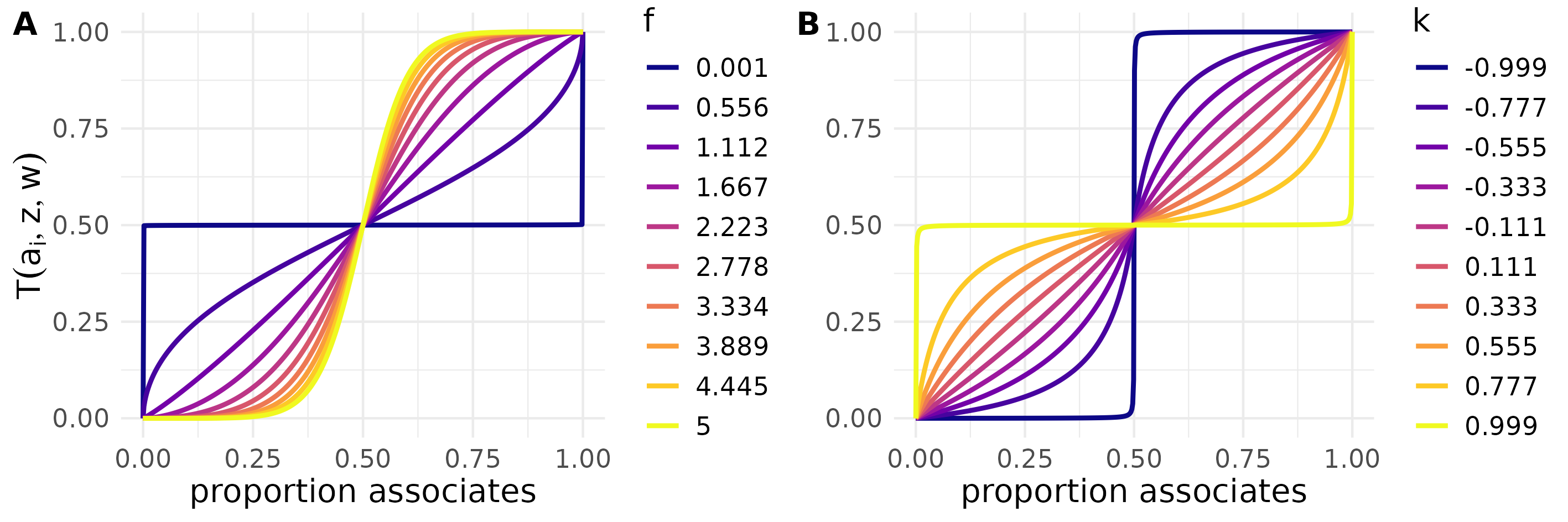
You might find that one or the other has convergence issues, so we provide both. Complex transmission can be implemented with varying effects, ilvs, oada and ctada type models, etc.

Setting priors

You might want to customize the priors of your model. Here are the default priors:

default_priors <- list(
        log_lambda0 = "normal(-4, 2)", # intrinsic rate
        log_sprime = "normal(-4, 2)", # social transmission rate
        beta_ILV = "normal(0,1)", # beta coefficients for ILVs
        log_f = "normal(0,1)", # exponent parameter under freqdep_f models
        k_raw = "normal(0,3)", # k parameter under freqdep_k models
        z_ID = "normal(0,1)", # varying effects
        sigma_ID = "normal(0,1)", # SD of varying effects
        rho_ID = "lkj_corr_cholesky(3)", # LKJ prior for veff corr matrix
        gamma = "normal(0,1)" # gamma parameter for Weibull intrinsic hazard model
    )

To adjust any one of them, call generate_STb_model and provide a named list of those you wish to change in the priors argument. The distributions should be written with the usual Stan convention. You only need to supply those which you wish to change. For example, you might want to tighten your priors on intrinsic rate, social rate and beta params for ILVs.

data_list = import_user_STb(STbayes::event_data, STbayes::edge_list)
model <- generate_STb_model(data_list, priors = list(
     log_lambda0 = "normal(-4, 1)",
     log_sprime = "uniform(-4, 1)",
     beta_ILV = "normal(0, .5)"
))

At the moment, the function will always print all priors that are possible to specify, regardless of the type of model you are creating. At least this makes it easy to reference the names when you need them.

High-resolution data mode

If you have very high-frequency sampling of behaviour (e.g. from a motion capture system), you can take advantage of it to create a model with dynamic networks and dynamic transmission weights that can change in value frequently between events. Sampling intervals should be regular (e.g. 30 fps). Below is a dataset where networks and transmission weights are recorded every time-step, rather than summarized per inter-event interval. If fitting a model with standard transmission, STbayes preprocesses the data for efficient fitting.

data_hires <- import_user_STb(
    event_data = STbayes::events_hires,
    networks = STbayes::networks_hires,
    t_weights = STbayes::t_weights_hires,
    high_res = T
)
model_hires <- generate_STb_model(data_hires, transmission_func = "standard")

If you plan to fit a model with complex transmission, it’s not possible to pre-process the data because of the non-linearity of the transmission rule. You should use import_user_STb2(). High-res complex transmission models will take significantly longer to fit as they loop through each time-step, rather than inter-event intervals.

data_hires <- import_user_STb2(
    event_data = STbayes::events_hires,
    networks = STbayes::networks_hires,
    t_weights = STbayes::t_weights_hires,
    high_res = T
)
model_hires <- generate_STb_model(data_hires, transmission_func = "freqdep_k")

Import NBDA data objects

STbayes is compatible with most NBDA objects. The function will try to figure out what was meant to be done with ILVs. However, some features of STbayes require using import_user_STb. Below we read in an NBDA object (taken from Tutorial 4.1 from Hasenjager et al. 2021):

nbdaData_cTADA <- STbayes::tutorial4_1
data_list = import_NBDA_STb(nbdaData_cTADA)
str(data_list)